Building The Buffer Link Counting Service
On the surface the Buffer link counting service is pretty simple. Its job is to keep track of the number of times someone has created a Buffer post with a given url embedded into it.
An Example Link
{
  "url": "https://buffer.com",
  "created_at": "1480431305",
  "update_id": "123456",
  "profile_id": "654321"
}
Behind the scenes this is what powers the Buffer Button counts.

As we’ve recently shared, Buffer is moving towards a Service Oriented Architecture and moving the links counting logic into its own service. The links service accounts for a large portion of all Buffer API traffic and at the time of writing contains almost 600 million records.
Starting Out
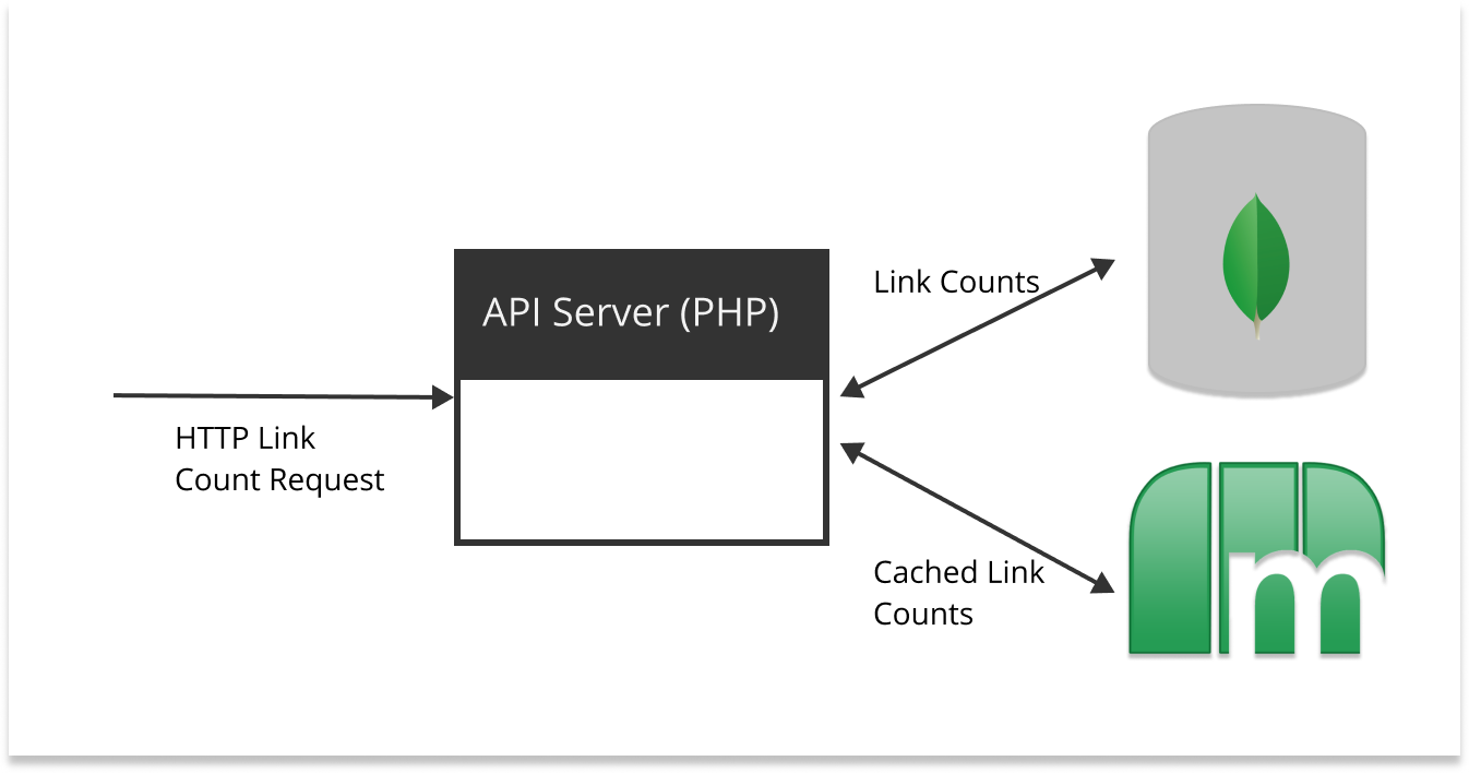
When I started working on the links service project, the production traffic was being served with a PHP backend and a Mongo database. There was also a caching layer stored in memcached.
Requirements
Aside from moving the links counting logic into its own service, we wanted to make sure the new service met the following requirements:
High Availability
The system should be able to tolerate a partial failure. If one links service replica goes down, the system should still service requests on the other replicas. This means that building a stateless, or even more specifically, conforming to the 12 factor app principles is key.
Handle High Throughput
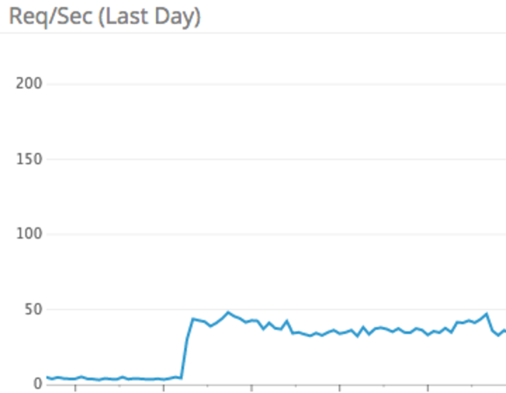
After collecting data from the original links service we found an average of 400 req/sec with bursts upwards of 700 req/sec. On the write side we observed 8 inserts/sec from the workers. Indicating a heavy skew towards read. We should not only be able to handle the current workload, but handle future workload as it increases (making the assumption that this feature gets utilized more over time).
Maintain Historical Data
The links service collection contains time series information that could be utilized in future features. We wanted to preserve the data even though we wouldn’t need it directly for the counts.
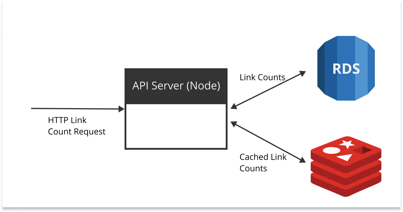
Iteration 1: Amazon RDS (Aurora) + Node + Redis
Amazon RDS (Aurora) is a MySQL compatible database that has some nice features like auto-scaling and a simple interface to increase compute power. We decided to go with RDS - Aurora for a number of reasons:
- High throughput
- Data autoscaling
- MySQL in local dev environment
Node almost needs no introduction. It’s server side JS backed by a powerful packaging system. It’s an async powerhouse driven by its event loop. We chose Node for the following reasons:
- Thriving community
- Package manager
- Handles lots of async I/O (request handling and db requests)
- Pretty simple to containerize
Redis is an in-memory data store that can be used as a database, cache or message broker. It has capabilities to operate in a cluster with replica sets, which is a huge plus if you’re looking for high availability. We decided Redis was ideal because:
- Cluster mode and replicas for high availability
- Reads are lightning fast
- More flexibility around caching
- AWS offers managed Elasticache Redis
Combining these technologies together, we decided on an architecture that looked like this:
After backfilling the records and setting indexes we ran some test queries.
SELECT count(*) WHERE url = 'buffer.com'
The idea here is to count the number of times buffer.com has been shared. This works well so long as the counts for given urls are relatively low (> 200K).
When running a count on a url with a result in the millions, queries were taking 20+ seconds even with the URL field indexed. This was especially concerning, since there are a couple URLs with counts in the 80-90 million range. Running EXPLAIN on the query shed some light onto the problem:
SELECT count(*) WHERE url = 'popularurl.com'

--

4200000
EXPLAIN SELECT count(*) WHERE url = 'popularurl.com'

--

key | rows
----------
url | 5000000
Explain returned that in order to calculate the exact count it needed to scan through 5,000,000 records. Granted this is better than a full table scan of 600,000,000 records, but is still going to take some time.
With larger datasets, MySQL is really good at finding a needle in the haystack (one person’s profile data for instance). But it’s not great at answering questions like “how many pieces of straw are in the haystack?”.
We decided to keep iterating.
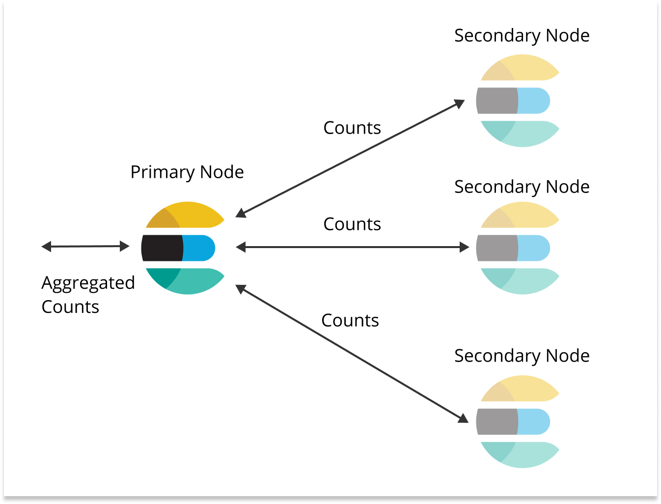
Iteration 2: Elasticsearch
Elasticsearch is a search engine built on Lucene. Elasticsearch search allows you to distribute data across shards and shards are distributed across nodes (along with replicas). So when you run a count query, the query is sent to each shard (and replica). When each shard has completed the count, the counts are aggregated on one node. This style of counting is very much like a map -> reduce job on other frameworks, which is very powerful because the load is distributed across nodes.
Some reasons we chose Elasticsearch:
- Query mechanisms are better tuned to our use case
- Cluster allows for high availability
- Elasticsearch in local dev environment
- AWS offers fully managed cluster
After backfilling we ran some test queries using the Node count API. Initial results were very promising, as we where seeing response times in the 100 - 200 ms range for all urls tested. So we decided to roll out the new service at 1% of the production traffic.
Things were looking great at 1%, so we stepped up to 10% and then 50%. Oops, we broke it. Requests jumped up to 15 seconds (error timeout) and the containers on Kubernetes started running out of memory and eventually would get killed. After some investigation, we determined that Elasticsearch was the bottleneck. We started trying to optimize the query by using filters so we could utilize the Elasticsearch cache. At this point the thought occurred that this might not be the best solution for our workload. “We’re at 50% of our current workload and we’re already doing query optimization”, which seemed troubling since we wanted to build something that could carry us into the future. But there was still more unknowns to explore before giving up on Elasticsearch.
The next thing we tried was to add another replica to the links index. We were looking to increase the read capacity of the cluster and the Elasticsearch docs call out that one strategy is to increase the number of replicas. However, adding the replicas caused the queries to return more slowly.
Let’s say for a minute you’ve got one node, one shard and zero replicas. Now let’s say you run enough queries on the index to use 100% of the resources on the node.
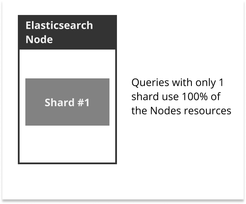
Now lets say you set the replicas on the index to 1 and run the same queries as with the previous experiment. Elasticsearch is going to run queries on both the shard and the replica, effectively splitting the node’s resources. Keep in mind with the previous experiment caused the node to consume 100% of its resources. Splitting the resources under heavy load would cause the queries to take longer.

Keeping the replicas the same and increasing the number nodes would have been the better solution in our case. However the Elasticsearch cluster was already large enough to be more expensive than our Mongo database. It became clear at this point that changing replicas and nodes would not be enough to carry us confidently into the future.
So again, we decided to iterate.
Iteration 3: Redis + S3
Our strategy of storing the links in a collection had proven to not be scalable. Every count on the links collection was doing a massive amount of work. So we decided to rethink our data structure to better suit our workload.
We ended up decided to use a simple hash data structure to store counts:
{
  "buffer.com": 5000,
  "popularurl.com": 4000000
}
As with any decision with data structure there’s some tradeoffs you have to make. When you store links in this way it’s more difficult to recover from error states because you’ve got no history. With a counter you have a snapshot of the world, rather than the historical view for all time. To compensate for this drawback we decided to archive the links in S3 with the previous data structure, that way we could backfill another service or recover the links service in the event of a catastrophic failure.
What you get in return is the ability to leverage work you’ve already done, rather than repeating large amounts of work over and over again. Your current snapshot is a superposition of all previous states of the system. To update the snapshot, a simple increment operation is enough to merge all previous states with the current change - meaning that both reads are writes are very fast!
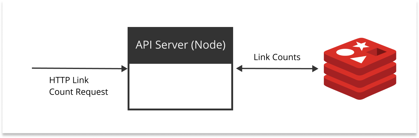
We decided to use Redis as our main datastore, with a simplified architecture:
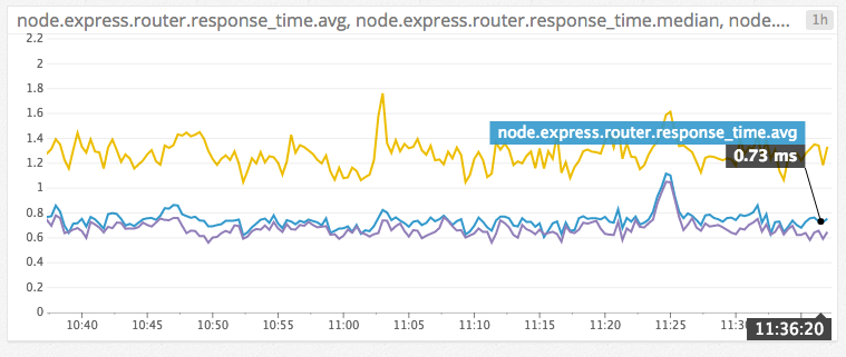
After backfilling we ran some test queries and were blown away by the performance - sub millisecond response times! We decided to move forward with 1% of production traffic.
Things were looking great at 1%, so we increased traffic to 10%, then 50%, then 100%. Even with 100% of production traffic, average response times stayed below one millisecond.
At this point we were all convinced we had applied the right data structures and tech stack to support our link service customers well into the future. We even had some options that were unavailable in the past, things like realtime counts (we cache responses with our CDN for 10 minutes). We could also use the historical S3 data to backfill future services to support feature we could only dream of. So many possibilities!
Reflecting
Sometimes things look very simple on the surface, even if you’ve done similar projects. It’s only when you’ve dug deep into the implementation and ran experiments (likely in production) that you find out if something is going to work. I think it’s one of the paradoxes that make building software interesting. Challenging assumptions until you figure out whats lurking beneath the surface (thar be dragons). It’s been an epic journey building out the Buffer links service, and I hope that sharing these experiences with others will be helpful.
Have some thoughts on this? Reach out to me on Twitter: @hjharnis